These Doodle Insights are brought to you by my super generous patrons on Patreon!
One month ago, I had an idea. Could I modify my tiny Pico-8 voxel engine to have it in a first-person view, with a small world to explore?
Today, I’m releasing this Pico-8 first-person voxel game called Lands Of Yocta, which is also very much a tech demo showing off my latest advances in Pico-8 voxel technology! If you haven’t already, you should check it out before reading any further!
And in this very special and very long Doodle Insights I will be describing each step in the development from where we left off in the Doodle Insights #12 to this final first-person voxel game.
All of these steps were the subject of a Twitter thread of gifs which you can check out if you want a visual taste of what you’ll be reading here!
Exhibit A – The Starting Point
This is basically what we had at the end of the Doodle Insights #12. If you haven’t already, I really think you should read it before continuing on this. But if you don’t want to do that or if you need a reminder of what we saw in the Doodle Insights #12, here is the end summary from that:
Voxels can be drawn as squares and no one will notice at first glance! You only need a little maths to find the projected coordinates of all the voxels on your screen! The drawing order of the voxels is super important but can be managed quite easily! Store your voxel data in the sprite-sheet and you can modify it at runtime like it was nothing! The whole thing can be optimized by putting the voxel data in a table rather than in the sprite-sheet directly! Have fun with the code and you could end up with a tiny-TV on which you could play awesome tiny games!
A forest seemed like a nice type of place to explore so I went for that. At this point, the voxel data is drawn in the sprite-sheet as 16×16 layers and the code puts it into a structure of tables for quicker access at runtime.
Exhibits B, C – 3D Maths Is Horrible


Unless you discovered me through my voxel stuff, you know me for my 2D games and doodles. Even when I do 3D renders, I almost always cheat somehow. The reason for that is that I don’t like 3D. In my opinion it makes both programming and design much much more complicated, just because you always have to consider that third dimension. I’m also convinced there’s still much unexplored ground in 2D which is why I still make video games anyway. But it had been a while since I last worked on a 3D project and it was somewhat nice to get back to it with this project. At least at first.
But 3D maths is just horrible. You have to draw out weird 2D representations on sheets of paper and even with that it can get painfully confusing.
These two exhibits are me trying to figure out this first person camera thing.
While I have no idea what’s happening with Exhibit C, Exhibit B is actually much closer to what I wanted. (except for the fact that it is upside down)
Even though each cell is still represented by a 4×4 square, depth has been added and helps define where each cell should be drawn and if it should be drawn. Because obviously if a cell has a depth lower than zero, it means it is behind the camera and should not be drawn. (otherwise you may get some strange results)
The depth itself is based on the algebra previously used to calculate the y position of each cell. If we consider the x position as the cosinus of an angle, the depth is nothing more than the sinus of that same angle. (it is actually a bit more complicated that that, especially as we really don’t want to do trigonometry on every single cell, but it’s the idea)
Exhibit D – We Did It!

The dimensions of each voxel square now depends on the depth!
We also made the depth influence the x,y position of each cell on the screen more, to get that nice and immersive zoomed-in effect.
Here’s the algebra behind the scale of the cells based of the depth by the way:
scale = -d/24*1.8+4
This will prove to be very wrong later on.
But something else that is not necessarily apparent needed to be done. In our old view, the layers of voxels could simply be drawn from the lowest one to the highest, so the higher levels would be drawn above the lower ones. But now, the camera has layers under it and above it and keeping the old drawing order would make half the screen look weird with the wrong layers being drawn above the right ones. Here’s how we handle that:
for ll=0,15 do
 local l
 if ll<8 then
  l=ll
 else
  l=15-(ll-8)
 end

 --draw layer l
end
Also, let’s quickly mention that in the current version of Pico-8 (0.1.10c) and previous ones (probably), there is an exploit that lets you draw rectangles without any CPU cost at all. It’s very easy to do: when calling ‘rectfill(x1,y1,x2,y2)’ you want to have either x1>x2 or y1>y2. It’s very likely that the CPU cost is calculated on the surface of the rectangle but does not handle variables not being in the right order. This exploit will probably get fixed in future versions and it is not being used here nor in any of the other Exhibits, nor in the final game.
But hey look it’s voxels and there is a first-person type of camera, that’s what we wanted, so that’s it we’re done right?
We’re not done.
Exhibits E, F, G: “Frustum Culling”


I wanted to display more. I knew I could because there was some free CPU left and I had an idea of how to display just the cells we want on screen.
Frustum culling is a technique used in regular polygonal 3D that consists of only rendering things that should be in the screen. Any off-screen object is simply excluded from the rendering phase, for the sake of performances.
We’ll take inspiration from that and figure out exactly what cells of our scene should be rendered and only render these!
So we have to define what portion of some sort of map we want to render. The map will be the same voxel data repeated over and over again and for any cell, the data will be at ‘_vox[z][y%16][x%16]’. Because we can’t look down or up, we don’t need to care about anything more than a top-down view when thinking about this.
To define this portion, we need at least three points: the camera position, the furthest point to be rendered on the left border of the screen and the furthest point to be rendered on the right border of the screen. And we will be adding the furthest point to be rendered in the middle of the screen, so the outer reach of our rendering looks a bit more like an arc.
Those points are really easy to find, here’s how it goes:
--in the draw_voxel() function
local dist,da=55,0.05
local x0,y0=round(posx),round(posy)
local x1=round(posx+dist*cos(cama-da))
local y1=round(posy+dist*sin(cama-da))
local x2=round(posx+dist*cos(cama))
local y2=round(posy+dist*sin(cama))
local x3=round(posx+dist*cos(cama+da))
local y3=round(posy+dist*sin(cama+da))

local pts={{x0,y0},{x1,y1},{x2,y2},{x3,y3}}

--that's my round function, it's somewhere else in the code
function round(a) return flr(a+0.5) end
‘dist’ here is the drawing distance, the maximum distance at which we’ll render cells. ‘da’ is the view angle (it’s a thing if I say it is) at which are considered to be the points on the left and right sides of the screen from the center of the screen. The points calculated are the corners of the shape drawn in Exhibit E.
Let’s talk some more about that Exhibit E. We’re drawing the shape between the four points there. That shape is convex and it happens that convex shapes can be drawn with code from our friend Jakub Wasilewski!
Jakub is currently making this game called Dank Tomb, which is also a tech demo (a 2D one) but it should actually end up as a really fun game! He also wrote 4 articles about what makes it such an impressive tech demo: his lighting. The articles form a bigger tutorial in four parts which you can read here, here, here and there. But only the 4th part is of interest to us as that’s where he shows us how to draw convex shapes.
Here’s some key stuff that I’m stealing directly from his article:
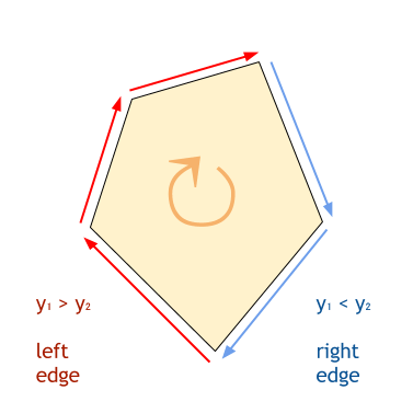
ymin, ymax = Y coordinates of the top/bottom of the polygon
for each y between ymin, ymax:
 xls[y] = find the leftmost x still inside the polygon at line y
 xrs[y] = find the rightmost x still inside the polygon at line y
for each y between ymin, ymax:
 fill(xls[y], xrs[y], y)
(it makes more sense in the article, you really should read it now or later if you haven’t already)
This is what’s used to draw the shape in Exhibit E but it is also what’s used to find the cells that should be rendered in Exhibit G. (and Exhibit F but that one was just my first clue that my depth scaling was slightly off)
Just as we would draw lines of a convex shape, we are rendering lines of our frustum-culled area. (it’s a thing if I say it is) And of course the drawing order was the next tricky thing there.
For our y loop (in the voxel drawing loop structure), it’s alright. We have our ymin and ymax values and these will serve as ystart and yend in our ‘for’ loop. The ypace (1 or -1) is decided by looking at the camera angle just as we used to do it in the Doodle Insights #12.
For our x loop, we have a xmin and a xmax for each line (xls[y] and xrs[y] from Jakub’s pseudocode). We can’t decide which is start and which is end for each line before going into the loops, that would cost as much CPU as doing it inside the loops. But we can decide of the order as it will be the same for every y line. Something else we can do is storing them as xmin and xmax in a tiny array just as we get to the x loop, and then use these values as loop parameters by using array indexes! Here’s what it looks like:
local ystart,yend,ypace
if cama%1>=0.5 then
 ystart,yend,ypace=ymax,ymin,-1
else
 ystart,yend,ypace=ymin,ymax,1
end

local xstart,xend,xpace
if cama%1=0.75 then
 xstart,xend,xpace=2,1,-1
else
 xstart,xend,xpace=1,2,1
end

for ll=0,15 do
 --[...]
 for yy=ystart,yend,ypace do
  local xorder={lxs[yy],rxs[yy]}

  for xx=xorder[xstart],xorder[xend],xpace do
   --draw cells
  end
 end
end
The draw order was restored.
Exhibit H – We Did It???
Back to our first-person view!
In Exhibit G, we went back to the old isometric-ish view (it’s actually called “anometric projection”, I googled it) for visualization purposes but now it’s time to come back to our first-person view with depth scaling and… oh.
As you can see, we have our first person camera, the frustum culling works well and we can actually render things pretty far! I even made it so we control the camera and we can move!! But something is off.
Our depth-based scaling algebra is actually very wrong, in that it takes a really bad approach to 3D projection maths (even the name sounds boring to me) which was to try the first thing that comes to mind and see if it looks ok. Anyway, let’s fix that algebra.
Exhibit I – Pico-8 Doodle #75
scale = -(1/d)*48
It was as simple as putting the depth variable on the other side of the division symbol! This actually gives us something that looks slightly more like actual 3D projection maths with a FOV and all that boring stuff! (I think)
At this point I also remade my 16×16 voxel scene, leaving only one tree and adding a mushroom and a rock! The grass is different too. The voxel data now only has a few grass blades, the rest is just the lower half of the screen being colored in dark green, while the upper half of the screen is colored in light blue for the sky. The less voxels to draw, the more CPU to render voxels.
And let’s get even more CPU back while we’re at it! We saw in the Doodle Insights #12 that it was better to have our voxel data in a table structure so we could access it with _vox[z][x][y], rather than sget() which is slow. But that’s still three accessor calls in _vox[z][x][y], Pico-8 has to get into each level of the table structure every single time you use it. At the deepest level of our voxel rendering loops, this is inefficient and unnecessary.
Instead, we want to rearrange the voxel data structure so that it corresponds to our drawing loops structure. At the beginning of each loop, we’ll get the corresponding level of the data structure and save ourselves the accessor-call deeper in the loops. Here is what it looks like:
for ll=0,15 do
 local l --[...] we've seen that before
 local lay=_vox[l]
 for y=ystart,yend,ypace do
  local lin=lay[y]
  for x=xstart,xend,xpace do
   local c=lin[x]
   --draw cell of color c (or not if c is 0)
  end
 end
end
The CPU thanks us and lets us have more voxels on the screen.
This marked a point important enough to call it the Pico-8 Doodle #75 and leave it at that for a few days.
Until the itch got too strong.
Exhibit J – A Small Repetitive World
It was possible to get an actual voxel world in this tech demo, possibly even an infinite one, I was convinced of that.
The voxel data for the previous 16x16x16 forest scene in the previous Exhibit was only taking a small part of the Pico-8 memory, which I always found larger than necessary. There was room for something bigger. There was room for pieces of something much bigger still.
Here comes the one system in this project that I’m super proud of: voxel tiling.
Even though my 16x16x16 scene took little memory space, simply augmenting the surface area would use up more and more memory at an alarming rate. And if you think about it, 3D games nowadays would never have a huge 3D model of a map with every objects already in it. Instead they would use assets and place instances of them. In 2D games, you rarely draw an entire level. You draw tiles and you place those.
8x8x16 voxel models would take near to no place at all individually, they would even be easy to make in the sprite-sheet, with one sprite line for each voxel tile. (so 16 sprites) When drawing the voxels, finding the right data for each cell would only be a matter of finding what tile the cell is part of.
That’s exactly what I did. Except that that last part is slightly more complicated than this.
We used to have our voxel data in a simple ‘_vox[z][y][x]’ table structure but now we have one more dimension for that table: the tiles. Here are our different possibilities:
_vox[t][z][y][x]
_vox[z][t][y][x]
_vox[z][y][t][x]
_vox[z][y][x][t]
We need to find which of these requires the least table accessing in the voxel drawing loops, in accordance with our previous table accessing optimizations, because when you have big loops like we do, it can amount to some really heavy CPU cost.
And the big winner is… ‘_vox[z][y][x][t]’!! (for now)
Our drawing loop now looks like this:
--inside layer loop
 for y=ystart,yend,ypace do
  local lin=lay[y]
  for x=xstart,xend,xpace do
   local ti=--[figure out ti]
   local c=lin[x][ti]
   --draw cell of color c (or not if c is 0)
  end
 end
In Exhibit J, we have ‘ti=(flr(x/8)+flr(y/8))%16’, which is pretty heavy but it’s ok because we won’t keep it.
On a different note, a compass appeared at the top of the screen! It’s cool to be able to tell which way you’re going!
To draw the cardinal directions on the compass, we calculate the angular difference between said directions and the current camera angle. That difference is multiplied and used as a position on the compass. The letter is drawn only if that position fits in the compass. This same process will also be used to draw indicators on the compass later on.
Exhibit K – A Less Repetitive World

In Exhibit K, we have a map called mapp (as to not mess with the Pico-8 map() function) and it is a 2D table structure initialized with random tiles.
At the deepest level of our drawing loops, we would have ‘ti=mapp[flr(y/8)%64][flr(x/8)%64]’ with 64 being the map’s width, if not for the fact that this is a double-table-accessor-with-division-and-modulo-and-flr() combo at the deepest level of our drawing loops and the CPU hates us now.
Luckily, there’s actually a really simple optimization, even though it feels a bit weird. We’ll make a look-up table for integer values of which we want the floored division by 8.
--this is in the _init()
flrs={} --naming things is hard
for i=0,511 do
 flrs[i]=flr(i/8)
end
64*8=512, with 64 as map width, we have a value for every cell’s x or y coordinate in the map.
This will genuinely be much better because simply accessing a table is already faster than calling the flr() function alone, the rest is bonus. Besides, this table will contain only numbers and that takes little memory.
But also, a second optimization is possible, one we already did too! We want to defer the table-accessings, each data structure level to its corresponding drawing loop level!
Here’s what it looks like now:
--inside layer loop
 for y=ystart,yend,ypace do
  local lin=lay[y]
  local maplin=mapp[flrs[y%512]]
  for x=xstart,xend,xpace do
   local ti=maplin[flrs[x%512]]
   local c=lin[x][ti]
   --draw cell of color c (or not if c is 0)
  end
 end
Much better!
Exhibit L – Back To The Forest
It was time to make some new voxel forest assets and drop the placeholder tiles that were used in the last two Exhibits. As you can see, the tile system works super well and is not that noticeable in-game! And there’s only 14 different tiles there. The memory is still plentiful and the view distance that the CPU lets us have is very acceptable.
We also changed the maximum height of the voxel tiles. 16 looked good but 12 seemed to be enough and having less layers to go through is just so much better for the performances. 12 will remain as the maximum height for voxel tiles from here on to the final game.
Exhibit M – The Forest Is Now Interactive
At this point I’m starting to look for the gameplay part of my tech-demo. The movement controls occupying all the buttons for the player one, I want a gameplay that doesn’t require any more buttons. So I made buttons to press in the game.
The tiles 14 and 15, last two rows of the sprite sheet as explained previously, are respectively a new button and a pressed button.
While our tile system is great for the voxel rendering, it turns out it’s also really good to check on individual tiles in our little world and modify them. Here’s what’s happening in this Exhibit:
--inside _update()
 --posx and posy are the coordinates of the camera/player.
 local x,y=flr(posx/8),flr(posy/8) --getting tile coordinates
 if mapp[y][x]==14 then
  add_shake(32) --screenshake
  mapp[y][x]=15
 end
It is that simple. Thank you almighty tile system!
Exhibit N – Starry Night Sky
Cool 3D demos have skyboxes. I too wanted a skybox. For those who don’t know, a skybox is the sky you see in the background when you play 3D video games. It is rendered as the inside of a giant box, whence its name, but we’re not doing that here so we don’t care.
We don’t have enough space on the sprite-sheet to store the four sides of a skybox. In fact we don’t have any place at all because it is all taken by the voxel data but let’s forget about that for a second and pretend we have a blank sprite-sheet to work with.
What we do have is more than enough space for a few individual star sprites. So we’re making those and we assign them to ‘star’ objects which will be stored in a ‘stars’ table. At first, every star has a random position in the 2D sky (think of it as a panorama) and then we make them repulse one-another a little so we have something more even. Final step is flooring all the coordinates so that the stars don’t flicker or move differently than others when rotating the camera in the game. We’re also adding a moon because we can and it looks good!
Just as for the compass, the position of the stars simply depends on the angle difference between the stars and the camera angle.
Ok, we have a cool night sky now. But what do we do about the voxel data that was in the sprite-sheet?
We compress it. A few days after starting this project, I made a sprite-sheet compressor, which you can check out on the Pico-8 BBS. Rather than copying raw sprite-sheet data into the code in order to have several sprite-sheets, I made a little program that could compress that data into a shorter string of characters and also decompress it at a pretty good speed. (depending on the complexity of the sprite-sheet) Using this, we can have our voxel data sheet as a shortened string in the code. To load it, we decompress the string into the sprite-sheet and load it into our table structure as usual. When we’re done, we use the line ‘reload(0x0,0x0,0x2000)’ to get our starry sprite-sheet back.
Does this mean we can have more voxel tiles? Yes, it very much does.
Exhibit O – Tile Animation
We know that modifying the tilemap at runtime is super easy so let’s push it!
In a new, compressed sprite-sheet, we made four new voxel tiles, composing four frames of an animated voxel spikes tile. In the code, spike objects are created and assigned to tile coordinates. Here is the update function of these objects:
function update_spikes(s)
 s.t+=0.01

 if s.t%0.15<0.08 then
  local v
  if s.t%0.3<0.15 then
   v=(16+flr(s.t%0.15/0.02))
  else
   v=(19-flr(s.t%0.15/0.02))
  end
  mapp[s.tiy][s.tix]=v
 end
end
I don’t think I can actually explain the maths that’s going on there but basically, we’re looking at whether the spikes are shooting or retracting and we find out which “voxel tile frame” should be placed. Then we place it.
Another thing that changed there is the view distance, which is now dynamic! At the end of the _draw() function, we use the value from “stat(1)” to check on the CPU usage. If it is under 90%, we increment the view distance and if it is over 95%, we decrement it. Yay for stuff that takes care of itself!
Exhibits P, Q – Dynamic Voxels


This was a tough one and it is not even used in the final game for lack of available memory to have a nice animated voxel character. The code is still in the engine/framework though and only needs to be used.
At this point, I thought the game would be an action game with baddies wanting to kill the sh*t out of you. First I wanted to draw the enemies as scaled sprites but I quickly realized I would have to place them into the voxel drawing order somehow and I went “no, let’s not do that”.
So I wondered if I could possibly incorporate voxel models into the voxel world, overlapping the voxel tiles, at runtime. At first I thought this was madness. But then I figured out it just might be doable.
In electronics, sampling is about recording or extracting a small piece of music or sound digitally for reuse as part of a composition or song, with or without alteration. (I googled it) Sampling is our solution.
Checking for overlapping voxel models when rendering our voxels would be way too costly, so we’re not doing that. We need to incorporate our voxel models into the existing tiles. But of course we will want to keep our original tiles unchanged. So we’ll need to duplicate them. None of these things sound very nice for our poor CPU, but you have to remember that one tile is only 12*8*8 cells which is manageable.
I could write a few long and technical paragraphs about this but I’m gonna try and keep it short instead, so as not to bore you off.
Any tile-sized voxel model being incorporated into the voxel world would occupy 4 tiles. (unless it’s aligned with the tile grid but let’s not care about exceptions) So 4 tiles will have to be sampled and modified with a part of the voxel model. Defining this “part” will be done by comparing the coordinates of the model to the tile grid. The untouched part of the original tile is directly copied from the original tile, while in the touched part we first check for the cells in the voxel model and only where we don’t find them, we get the ones from the original tile.
The 4 new tiles created from this process are incorporated into the voxel data table structure, just after the static tiles. Each modified tile is given a new index. We won’t bother to free them afterwards but instead, we will override them with new modified tiles every _update() so as not to fill up the memory with modified tiles.
There, that was the short version.
Exhibit R – A Whole New Drawing Order
Big idea. Let’s totally mess up the drawing order (which the whole project is based on) so we have the z loop as the deepest level of the voxel drawing.
A lot of the tiles do not go up to the maximum height of 12 (or even above 3 or 4) and yet the drawing loops goes through all the height levels anyway and use up precious CPU on it. But if the height dimension is at the last level of all our structures, we can think with voxel columns of various heights and handle them as such.
We’d go from _vox[z][y][x][t] to _vox[y][x][t][z] and we could create another table just for heights: _voxh[y][x][t]. That last table is filled up automatically when loading the voxel data for every tile. For each voxel column on each tile, we check what was the last cell in the column and we put its height in our height table.
A small complication is the drawing order (once again) of the cells in the columns. With our constant height of 12 and the layers as the first level of our drawing loops, we could easily figure out what layer should be drawn at the start of the loop. (we did that with Exhibit D) But we can’t do that anymore because deepest loop level and CPU.
However, there are only 12 different heights possible. So we’ll make a list of drawing order maps.
--inside the _init()
 local midhei=flr(vhei/2) --vhei=12
 lorder={} --naming things is hard
 for i=0,vhei-1 do
  local order={}
  for ll=0,i do
   if ll<midhei then
    order[ll]=ll
   else
    order[ll]=i-(ll-midhei)
   end
  end
  lorder[i]=order
 end
And here is our new drawing loop structure!
--in draw_voxel()
for yy=ystart,yend,ypace do
 local ty=yy%8
 local lin=_vox[ty]
 local linh=_voxh[ty]
 local maplin=mapp[flrs[yy%64]]

 for xx=xstart,xend,xpace do
  local d=--calculate distance from camera

  if d>3 then --if cell is in front of camera and not too close
   local ti=maplin[flrs[xx%mapwt]]
   local tx=xx%8
   local clm=lin[tx][ti]
   local mh=linh[tx][ti]

   --calculate things we can already calculate,
   --like depth-based scale and cell position
   --on the screen (or part of it)

   local order=lorder[mh]

   for ll=0,mh do
    local l=order[ll]
    local c=clm[l]

    if c>0 then
     --draw cell
    end
   end
  end
 end
end
Now this is getting pretty heavy but, like, what did you expect? Besides, this actually opened my eyes on yet some more optimizations!
First of all, you can see that we were able to defer most of the calculations one or two levels higher in the loop structure, which is good.
But also, up to now, empty cells have a value of 0. Why? Why do empty cells have a value at all? Probably because we didn’t think this through. Let’s fix that!
While loading the voxel data, we will now set empty cells as ‘nil’ which makes them disappear from the array. Our ‘if c>0 then’ check becomes ‘if c then’, which pleases the CPU. Bonus: empty cells no longer use up memory!
Of course, all these optimizations had to be spread to all the existing systems in the project, especially the new structure order. It took a while but by the end, our automatic draw distance had tripled. TRIPLED!!!
Exhibits S, T – Playing With Our Voxel Model System


We fixed our voxel model incorporation system according to the latest optimizations so I figured I’d try to see how far I could go with it. I couldn’t go very far actually but I still had fun.
In Exhibit S, we are conserving modified tiles instead of constantly overwriting them. It’s fun but Pico-8 blurts out an “out of memory” message just after the end of the gif.
In Exhibit T, I broke everything I think. I can’t exactly remember what happened but it looks like I messed with the wrong tile indexes?? I don’t have the code for these two anymore, so I guess we’ll never know.
Exhibit U – Your Classic Exploration Game Mysterious Cabin
It was time to make some new voxel tiles! On a new sprite-sheet I made 3*4=12 tiles for a cabin. It features cosy wooden walls, two windows, one with a curtain, a framed picture, a chair and a table with a mysterious object on it!
That new sprite-sheet was compressed and loaded just after the previous tiles. The memory is filling up but not too much yet.
You can see that this cabin is pretty heavy to draw for the CPU and the draw distance takes quite the hit. Sadly, I couldn’t think of any efficient way to optimize it without deoptimizing the other tiles. The cabin will remain as the CPU’s dread for the rest of the project.
But something else changed! If you’ve been looking closely at the gifs until now, you may have noticed weird artifacts in the voxel rendering at some camera angles. All this while, the drawing order has been looking wrong whenever the camera aligned with the x axis. The reason for this was that the drawing loops go y then x and the distortion caused by depth-scaling makes it look off at angles around 0 and 0.5. (to the east and to the west) But I understood that only at this point in the project.
The best solution I could find looks pretty terrible in the code. We are cutting our y drawing loop in two. One loop for one side of the x axis and another loop for the other side of the x axis. It’s ugly and it means we’ll have to do changes on both loops whenever we want to make any, but it works and most importantly, it doesn’t take up any more CPU than before.
Exhibit V – Round Voxels
What can I say, people love round things, that’s just a design fact. When I realized I could replace the rectfill() call drawing the cells with a circfill(), I immediately went for it.
And it did look pretty good! Although not quite as blocky which was an aspect I kinda liked in the old look. I was torn between keeping these new round voxels or going back to the blocky ones. So I asked Twitter…
“Why not both?” they replied.
Exhibit W – Garden And Chill
By expanding on our tile system, we can now have both rectfill()‘s and circfill()‘s in our voxel drawing!
Right next to the compressed voxel data, we have a new table: a list of all the tiles that should be rendered with circles. After loading the voxel data, we create yet another table in which we’ll map every single tile to either the circfill() function either the new square() function which uses rectfill() but takes the same arguments as circfill(). Instead of calling rectfill(x-w,y-w,x+w,y+w,c) in the drawing loops, we’ll call drawfoo[ti](x,y,w,c). We lost almost no CPU at all, apart from circfill()‘s being slightly heavier than rectfill()‘s, especially with big radiuses.
Other than that, there’s a whole new set of voxel tiles! I modified the voxel data loading so that I can have two or four tiles on the same line in the sprite-sheet. The new set of tiles contains 64 of them! The memory took a blow but it’s still standing because most of these tiles have a lot of empty space which doesn’t count, thanks to previous optimizations.
And 40 of these new tiles are actually voxel frames for animated water tiles! These work exactly like the spikes except that the animation is more straight-forward.
The old assets are either to be found in the new set of tiles or they completely disappeared from the project. The spikes in particular have been discarded as I decided that we’re making a peaceful exploration game.
Exhibit X – Mysterious Monoliths
More tiles! Since we’re making an exploration game, I want some environment diversity!
In a 128*128 map, four different zones are to be explorable in the final game. A swampy lush area where the player will be starting, a calm plain with the cabin, a forest, and a rocky plain with lots of small monoliths plus a big one.
I won’t be detailing the world generation here but you can take a look at the make_world() function in the code of the final game if you’re interested. It’s pretty straight-forward.
At this point, the plan is to have a special tile in each zone that would show you a piece of procedurally generated poetry and unlock the final ending.
Here, the bigger monolith is one of these special tiles and it makes your screen shake when you’re close to it, which is cool. The procedural poetry is not implemented yet though. (nor will it ever be)
Something more technical: wall collision has been implemented! (it was about time) It was fairly simple too, thanks to our almighty tile system! The “wall” tiles (including rocks, trees, water and actual walls) are listed in a ‘wall’ table. From this table is created a new table mapping every single tile index to a boolean of whether the tile is a wall or not.
When updating the player’s movement, we check on what tile the player will end up. If our table tells us this tile is a wall, the player must be stopped.
Exhibit Y – The End Is Nigh
More tiles again! Lots of tweaking on existing tiles too and tile animation by code! (as-in we are actually modifying the voxel tile’s data at runtime)
And guess what! All these new tiles nearly blew up the memory! It’s fine because it didn’t but it doesn’t leave us much room at all for procedural poetry. So we’re not doing procedural poetry.
Some more thought went into it and in the end I’m going with something simpler and somewhat more elegant. (at least in my opinion) The player has to find the monolith in each zone. Once the monolith is found and hugged, it mysteriously modifies its surroundings and teleports to the next zone. In the last zone, the monolith replaces the whole map with lots of glowing monoliths (animated by code), except for the cabin. Get back to the cabin and… get invited to read this very piece and awake from this weird hallucination you’ve been having. You’re back into the world (which is actually a newly generated one but shush), free to have a walk around, there’s no more monoliths to mess with you.
The game is basically done.
Exhibit Z – The Game Is Really Done

And this article is being finished.
In this last Exhibit, a title screen and ambiant sounds have been added. A few remaining small issues have been fixed, especially the occasional “out of memory” crash due to generating too much animated water.
In the end, I’m very happy with the tech-demo side of the game but less with the game side of the tech-demo. I achieved the chill ambiance I wanted but the interactive side of it with the monoliths is simply too short. But I’ve been working on this for a whole month. I want to work on other stuff now. It is time to put an end to this madness of a project. (besides I’m actually really happy with what I made anyway)
Thank you so much for reading along.
I don’t think I can do a summary as usual. But as a conclusion, let me tell you that Pico-8 is amazing and can be pushed to make super cool things simply by thinking with its limitations in mind. Learning and taking advantage of these limitations is partly what the Doodle Insights series is about and I’m super happy to be writing it!
This project has been quite something. There was a lot of back and forth and quite a few rewarding breakthroughs and a lot of worrying that I might not get to the end of it.
I’m very happy with it. And I’m very happy with this article too. But also, I’m happy to be done with this project so I can finally work on other things!
Note that the final game on the BBS is under CC4-BY-NC-SA license, meaning you can download it and modify it, create new tiles, make new worlds, make new systems, optimize it some more and then upload it again! (don’t sell it though) Just please mention me as the creator of the original voxel engine.
Thank you again for reading this whole thing!
And thank you so much to my Patreon patrons who support this series and have been very patient about this project blocking out some of the regular content! Here are their names!
Joseph White, Adam M. Smith, Ryan Malm, Matthew, Giles Graham, Luke Davies, Jake Meanwell, Tim and Alexandra, Sasha Bilton, berkfrei, Nick Hughes, Christopher Mayfield, Jearl, Dave Hoffman, Thomas Wright, Morgan Jensen, Zach Bracken, Cole Smith, Marty Kovach, GucioDevs, Anne Le Clech, Flo Devaux, Brent Werness, babyjeans, Emerson Smith, Cathal O’Keeffe, Dan Sanderson, Andrew Reist, vaporstack, Dzozef, Tony Sarkees, Justin TerAvest and Vorzam!
If you appreciate this project and want to see more from me, please consider supporting me on Patreon as well. You’d get some extra content and regular updates but mostly, you’d be helping me out a lot. And even 1$ per month helps a lot. (besides, wallpapers for 1$+ pledgers should be coming soon!)
Here’s a link back to the actual game/tech demo if you want to take a second look at it! (you can also download it or browse through the code with the buttons under the player)
Thank you for reading and enjoy the voxel tech!
TRASEVOL_DOG

You are a special human being
LikeLiked by 1 person
Как прочитать чужую переписку viber – взлом вайбер, взлом переписки вайбер.
LikeLike